Standard capture, CAD and SHP

Part 4 of 4 · Learning path · Sample counts

Start: the reviewed project from Part 3. Finish: turn Quick Capture off, save LDN-013, and verify CAD/SHP copies in a separate local project; the global project moves from 38 → 39 sites and 50 → 51 features.

Quick Capture is one collection option. This part of the global walkthrough uses the standard form, then shows CAD Manager and Shp Manager from export to a checked import.

Continue with the Mapplex demo workspace and fictional data in New York, London and Tokyo. The application stays in night mode with satellite imagery on the map. Phone screenshots lead the steps; the expandable examples use Mapplex's actual tablet mode, including its navigation rail and centered attribute editor. These are browser captures of the current application, not a native-device acceptance test.

Select any image to view it at full size. Refreshed form images recreate the original draft without saving it again; refreshed CAD/SHP previews were closed without repeating the imports. See the sample-count timeline when comparing earlier parts.

1. Choose the standard capture workflow

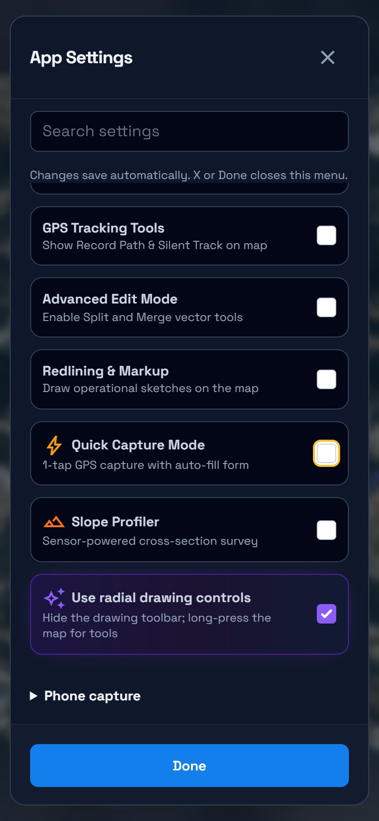
Open Settings → Field tools and turn Quick Capture Mode off. Choose Done. This changes the point-entry workflow; it does not remove the selected layer's form, required fields, Lexicon choices or configured spatial autofill.

Quick Capture is off. Radial drawing controls remain enabled; they are a separate choice.

Task	Workflow
Enter a point through the regular form	Quick Capture off → review location → Confirm Location → Enter Data → Save
Collect repeated points with Quick Capture	Quick Capture on and available → review location → Quick Capture form → Save Capture
Draw a route or boundary through the regular form	Quick Capture off → select a LineString or Polygon layer → draw vertices → Finish → Enter Data → Save

For drawing, keep Use radial drawing controls on to use the map's context menu. Turn it off when you prefer the visible toolbar and Draw Shape control. Quick Capture Mode and Use radial drawing controls do different jobs.

2. Place a point and complete Enter Data

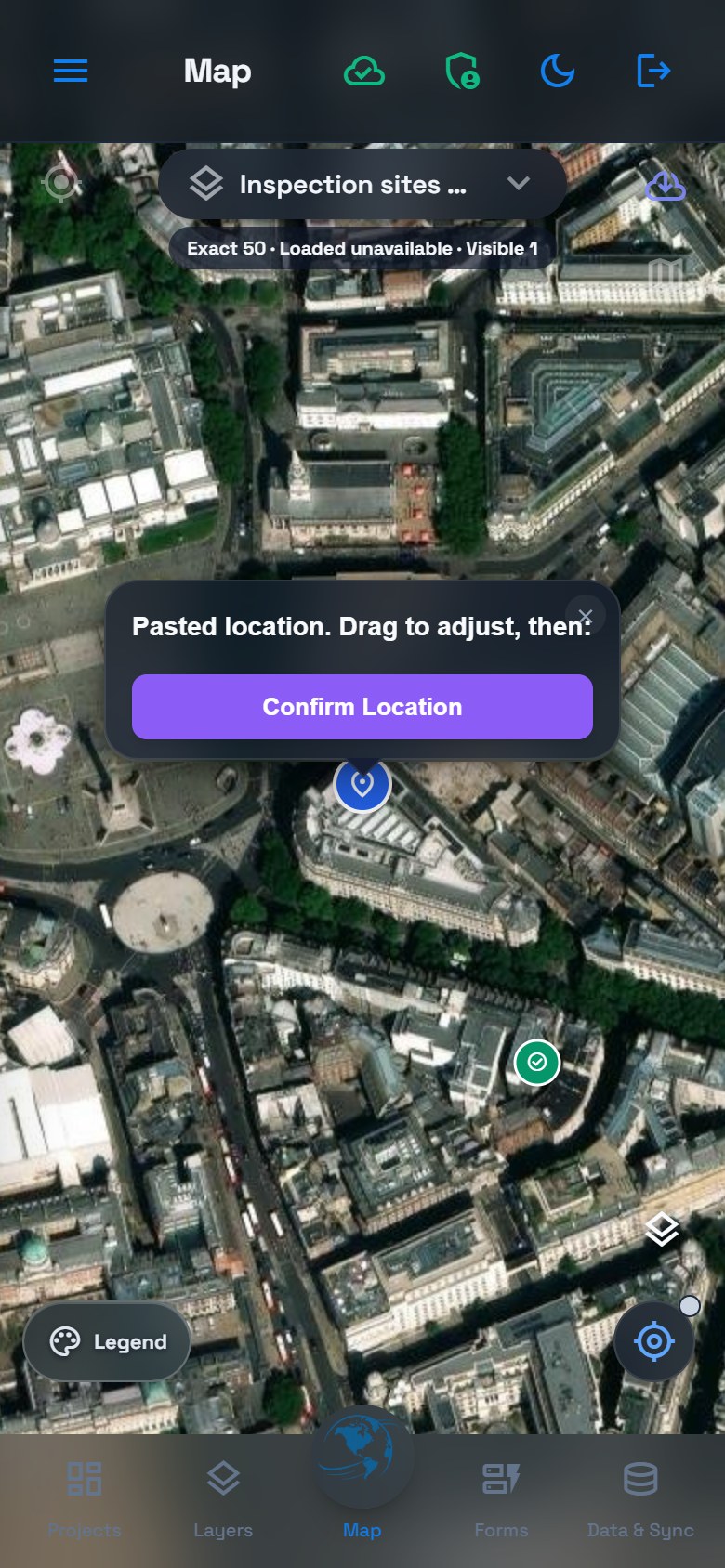
Activate Global Field Operations and select Inspection sites. For this repeatable London example, copy 51.5078, -0.1265, open the map's context menu on empty space and choose Paste Loc. It reads the clipboard; if access is unavailable, enter the same coordinate in the prompt. Review the temporary pin and choose Confirm Location.

This is a prepared training coordinate, not a GPS measurement. Confirming the pin opens the form; it does not save a record.

With Quick Capture off, the sheet is titled Enter Data. Fill in the inspection, then scroll through the remaining fields before Save.

Field	Example
Asset ID	LDN-013
Condition	Good
Height	7.2
Notes	Routine inspection complete. No repair required.
City	London
Service zone	London West, filled from the reference lookup
Inspection date	2026-09-09

The regular form still uses the layer configuration. Scroll down to review Service zone and Inspection date, then choose Save.

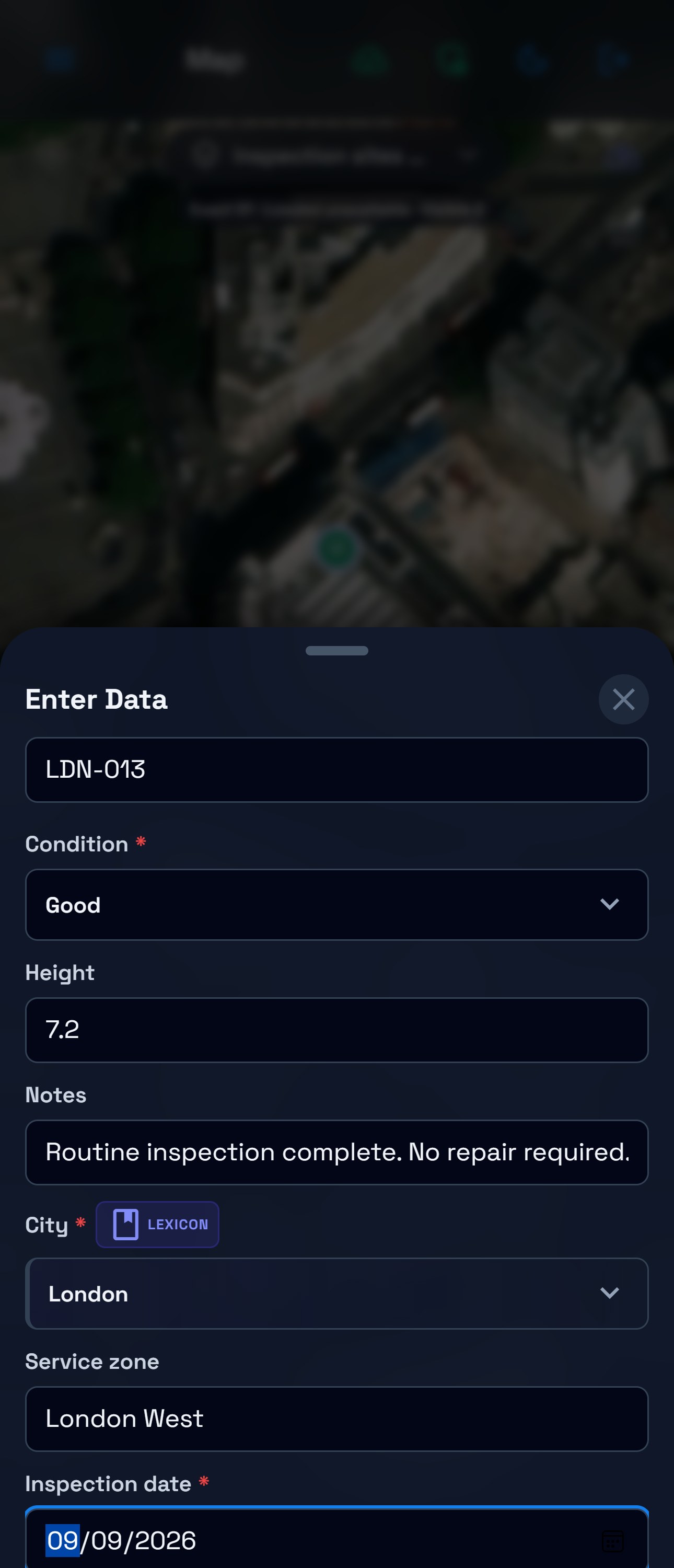
If a required value is missing, complete it and try again. Use Discard to abandon an unsaved draft. When repeating the exercise, choose a new Asset ID instead of creating another LDN-013.

For a line, add at least two vertices; for a polygon, at least three. Use Finish to continue to the attributes. The Precision crosshair and Snap to Features can help place vertices before finishing. See Contextual drawing for the complete route and boundary workflow. Turning Quick Capture off does not itself begin drawing.

3. Reopen and check the saved inspection

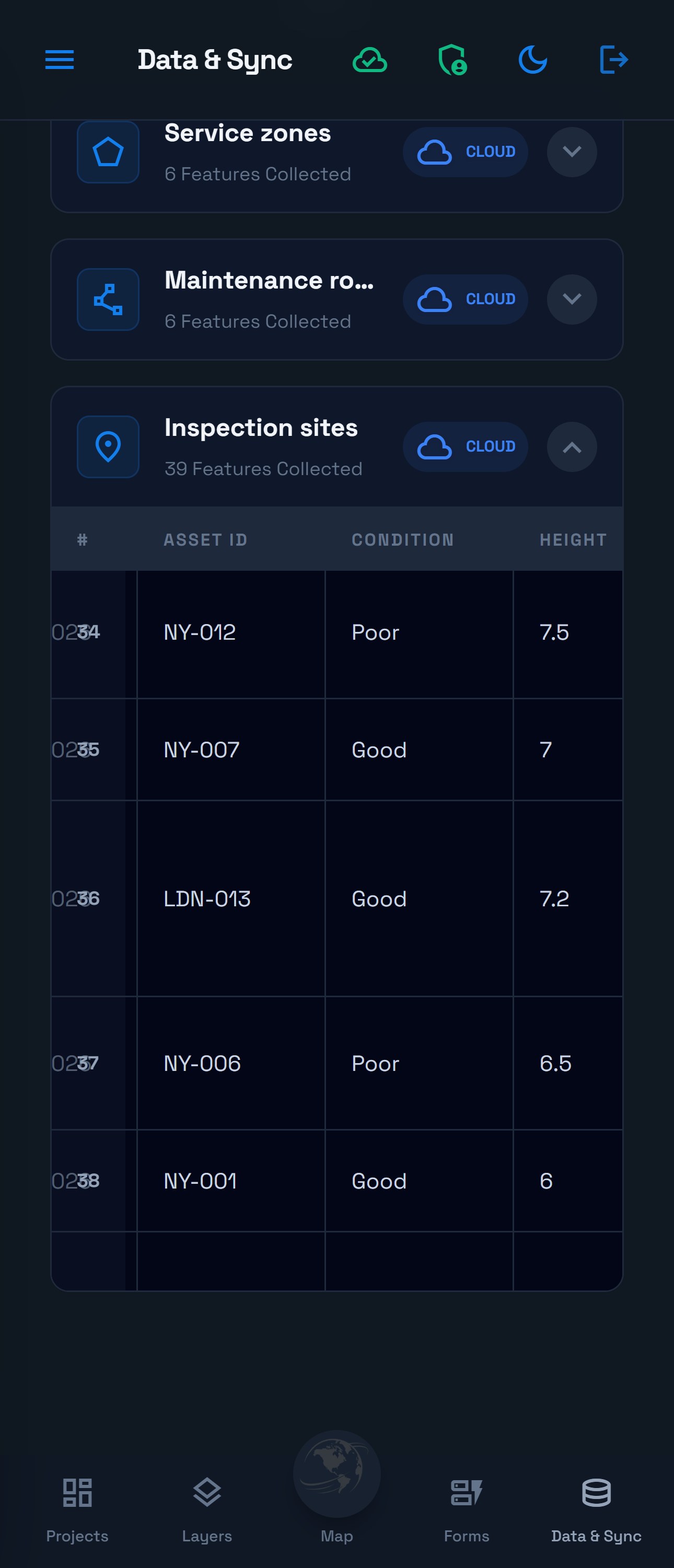
In Data & Sync, expand Inspection sites and find LDN-013. Swipe across the table to review its fields. The main project now contains 39 inspection sites and 51 features overall, including the existing six routes and six zones.

LDN-013 was saved once through the standard form and independently read back from the Geova backend.

On the map, open the saved feature's context menu and choose Attributes. The editor is now titled Edit Attributes. Review the values, then close the editor when no change is needed.

See the tablet mode view

The tablet presents a centered editor. London West and the other saved values can be reviewed without creating another record.

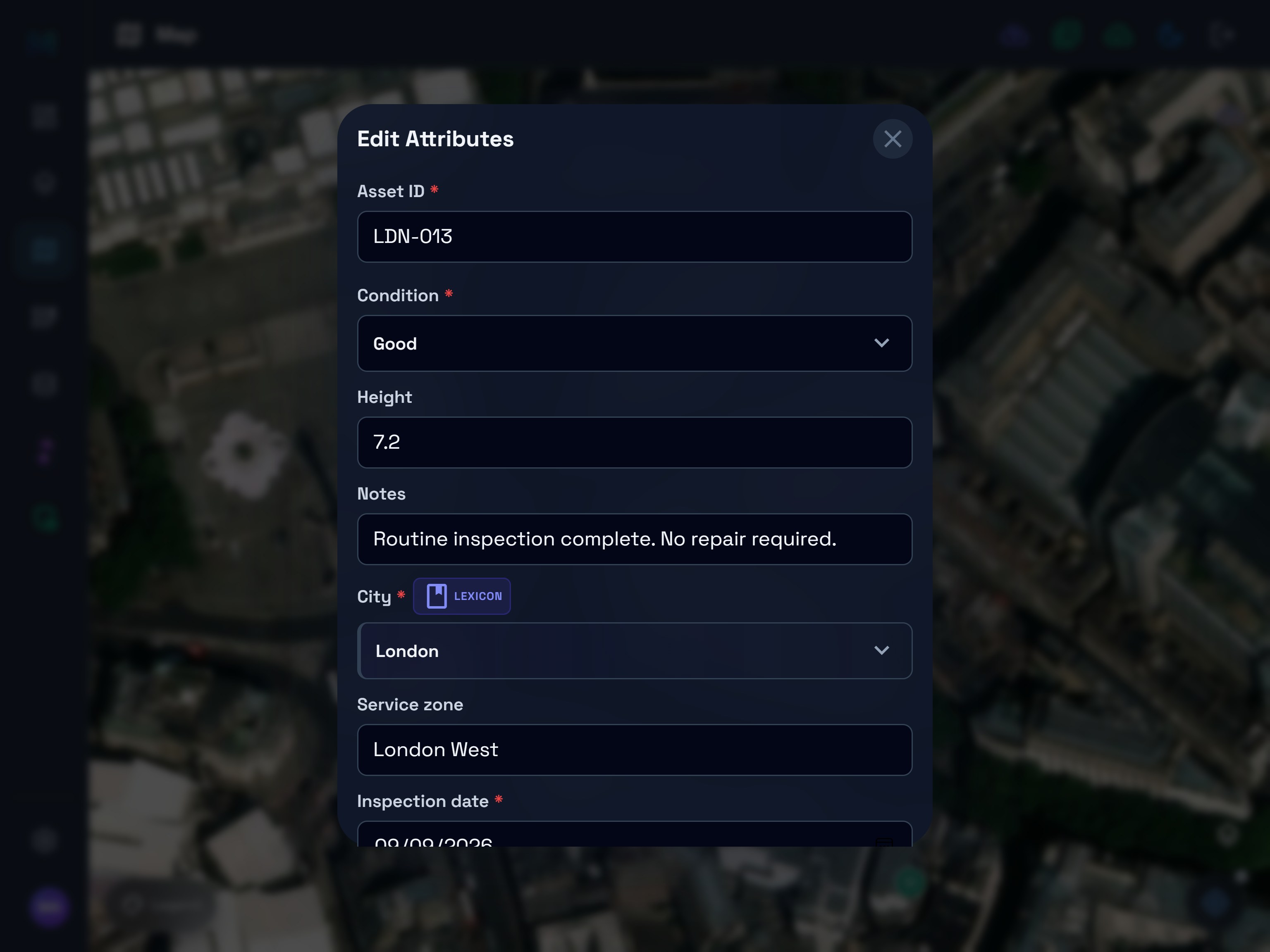
The City choice stores london through the Operating cities Lexicon. Older records may still contain the display label London. Use the delivery walkthrough when checking mixed codes, queued saves and export contents. A storage badge or map count alone does not establish delivery.

4. Export route geometry with CAD Manager

Open Data & Sync and scroll to the CAD and SHP launchers below the general import controls. Each opens its own manager. The workspace must include the relevant tool access; importing new layers also requires Owner, Admin or Editor access.

Choose CAD for DXF drawings or SHP for shapefile packages.

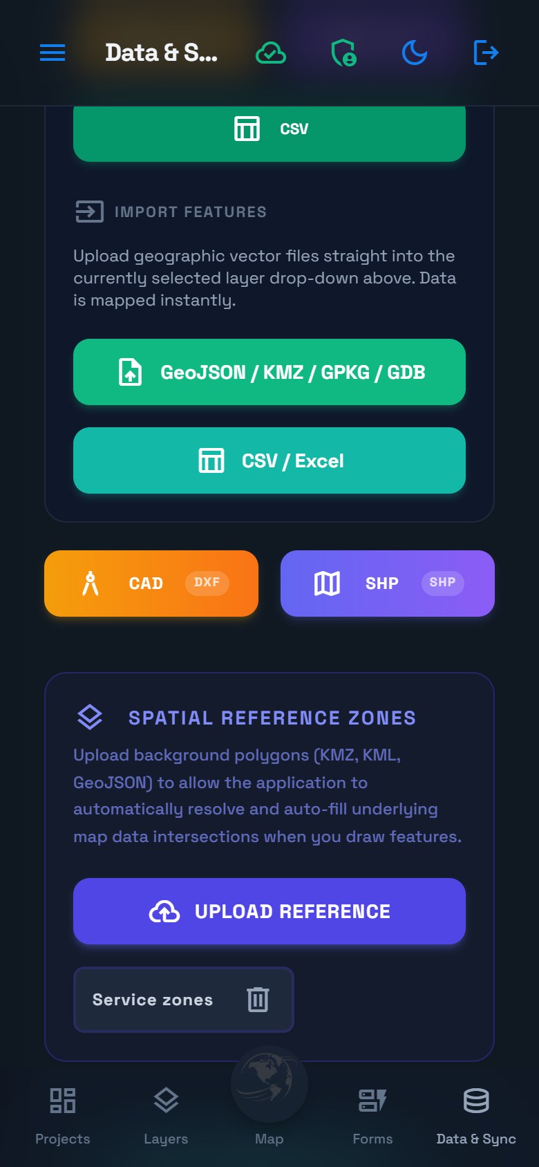
Open CAD → Export DXF. In the manager's own Select Layer control, choose Maintenance routes. For this global training file, keep WGS84 lon/lat (EPSG:4326) as the output coordinate system.

The manager has its own export scope. Check it even if a layer was selected elsewhere in Data & Sync.

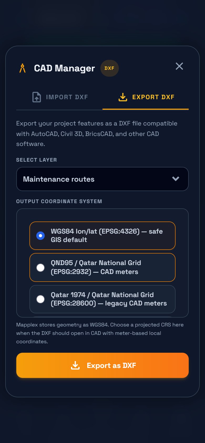
Choose Export as DXF and complete the download or device sharing action. This run generated a file containing six LWPOLYLINE entities, one for each source route.

The generated DXF was parsed and its six route geometries were checked through an actual reimport.

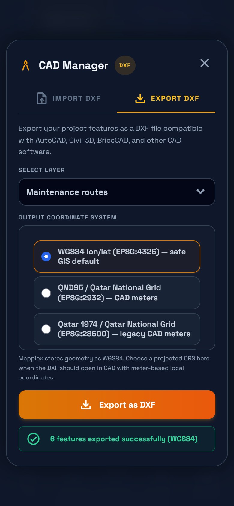
Choose units for the recipient. This example uses longitude/latitude degrees because it spans three distant cities. For engineering work that needs meters or a local grid, agree on the required projected CRS with the drawing's recipient. Do not choose a suggested local UTM zone or one of the listed Qatar grids merely because it appears in the menu.

DXF carries drawing geometry in this workflow. This export uses the CAD layer MAPPLEX_EXPORT and does not preserve the original Route ID, City, route status, form or condition styling. Polygon export writes exterior boundaries; it is not a complete polygon-hole or project-backup format. Use GeoPackage or GeoJSON when those data requirements matter.

5. Import the DXF into a practice project

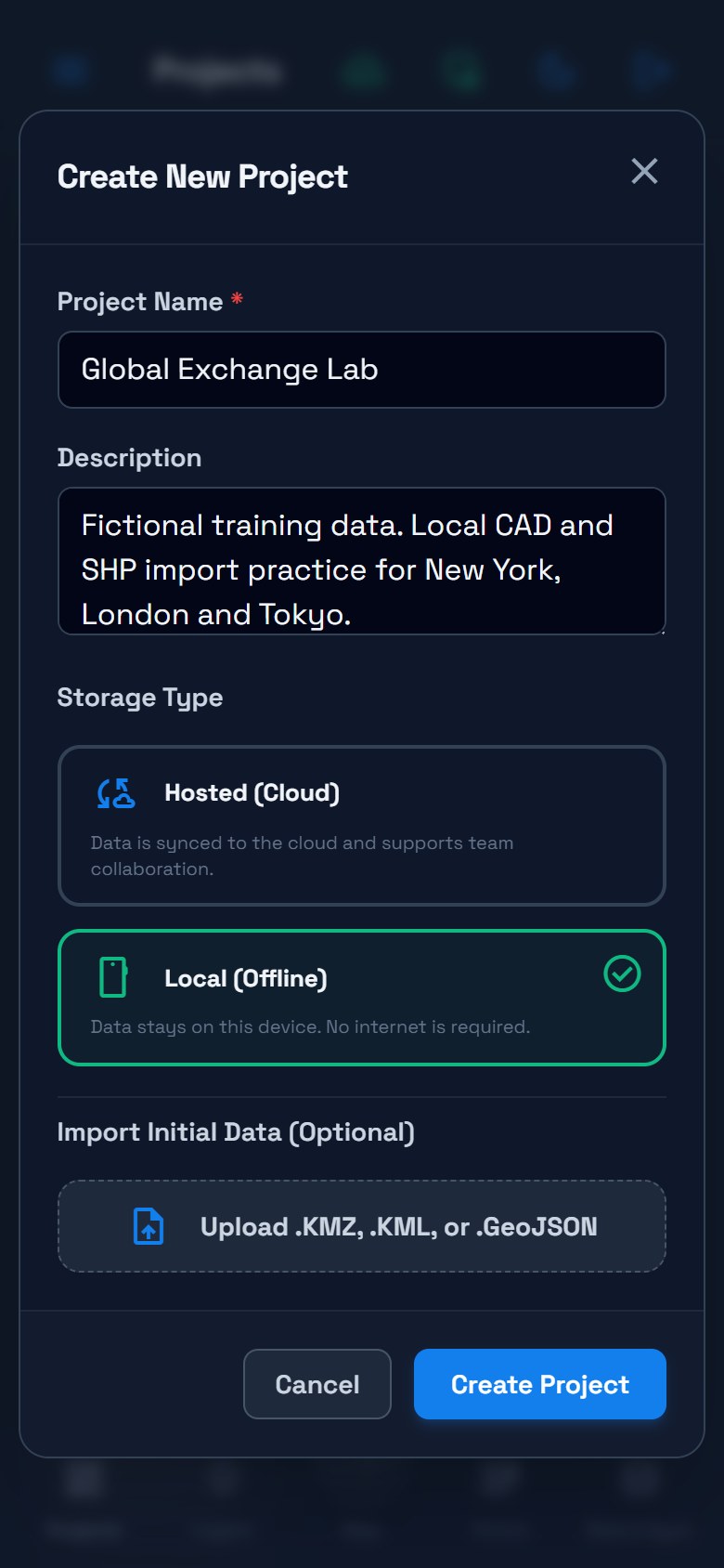
In Projects, create Global Exchange Lab with Local (Offline) storage for your first exchange exercise, then activate it before importing. If you are reviewing the prepared demo, open its existing lab and inspect the imported layers instead of importing the same files again. Use a new, empty local practice project if you want to repeat the full import.

Check the active project before each import: the lab receives the copies; Global Field Operations remains the export source. This keeps the practice data on this device.

The practice project is local. Its import results were not uploaded to the hosted Global Field Operations project.

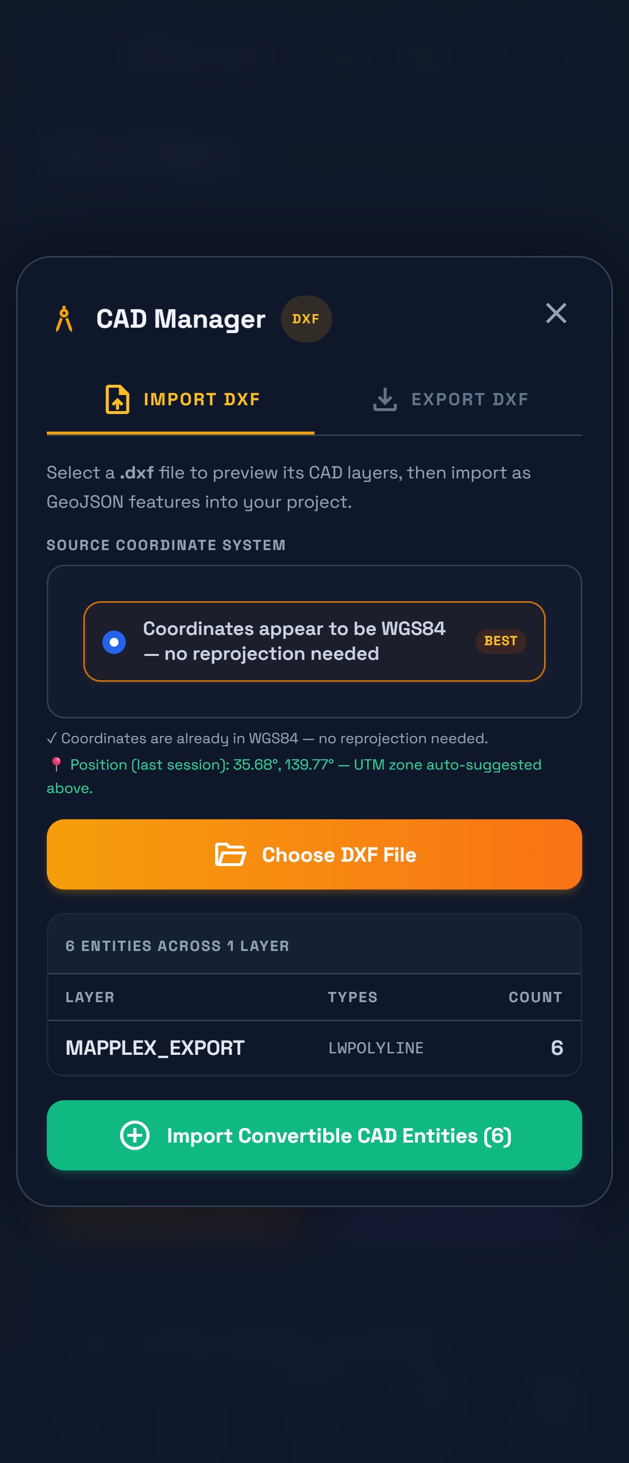
Open Data & Sync → CAD → Import DXF, then choose the exported DXF. Review Source Coordinate System, the CAD layers, entity types and convertible count. For this known WGS84 source, the preview says no reprojection needed.

A source-CRS suggestion is a check to review, not proof of the drawing’s coordinate reference system.

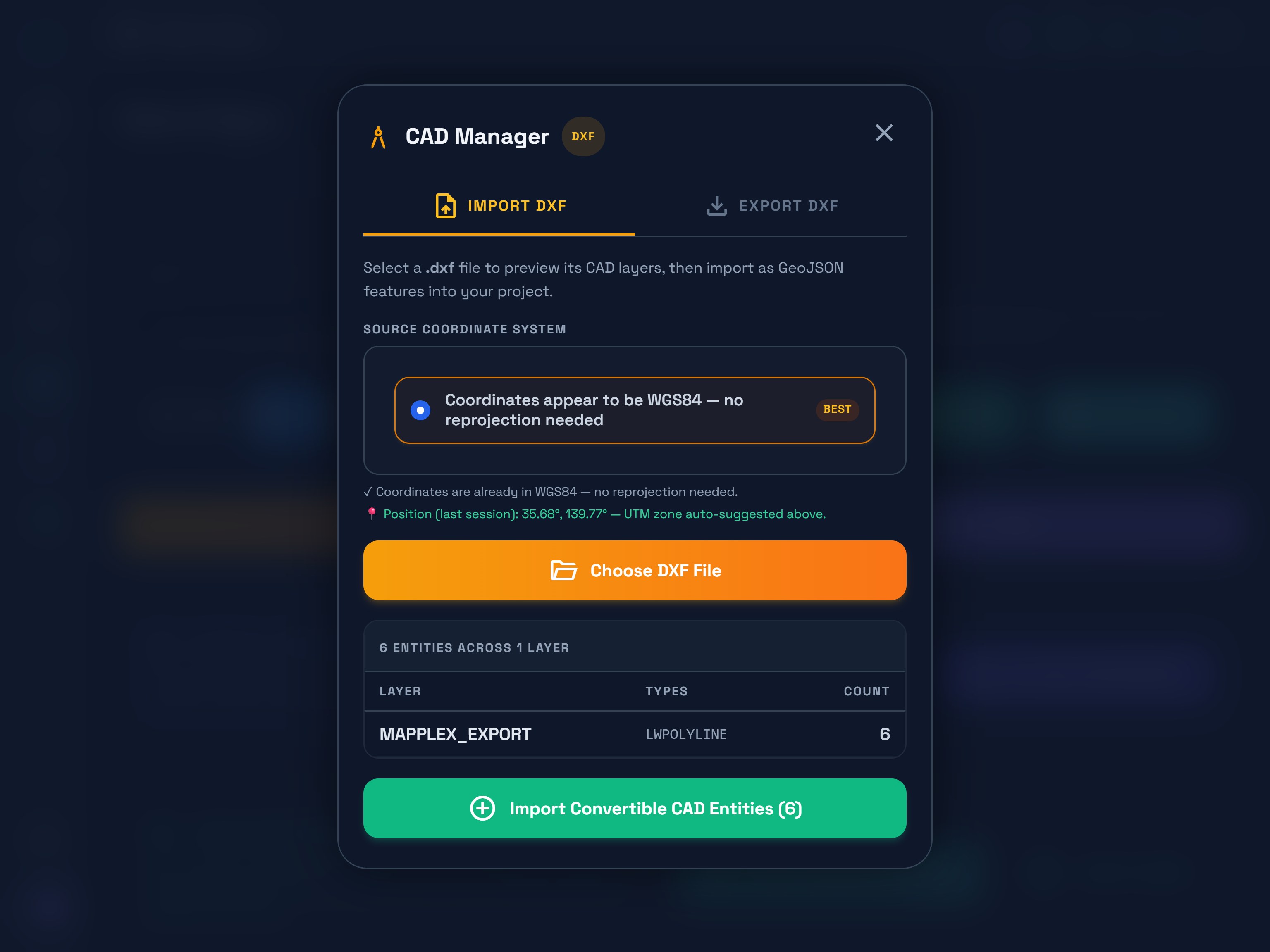
See the tablet mode view

The same preview and conversion choices are available in tablet mode.

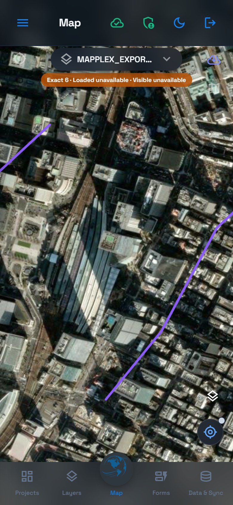
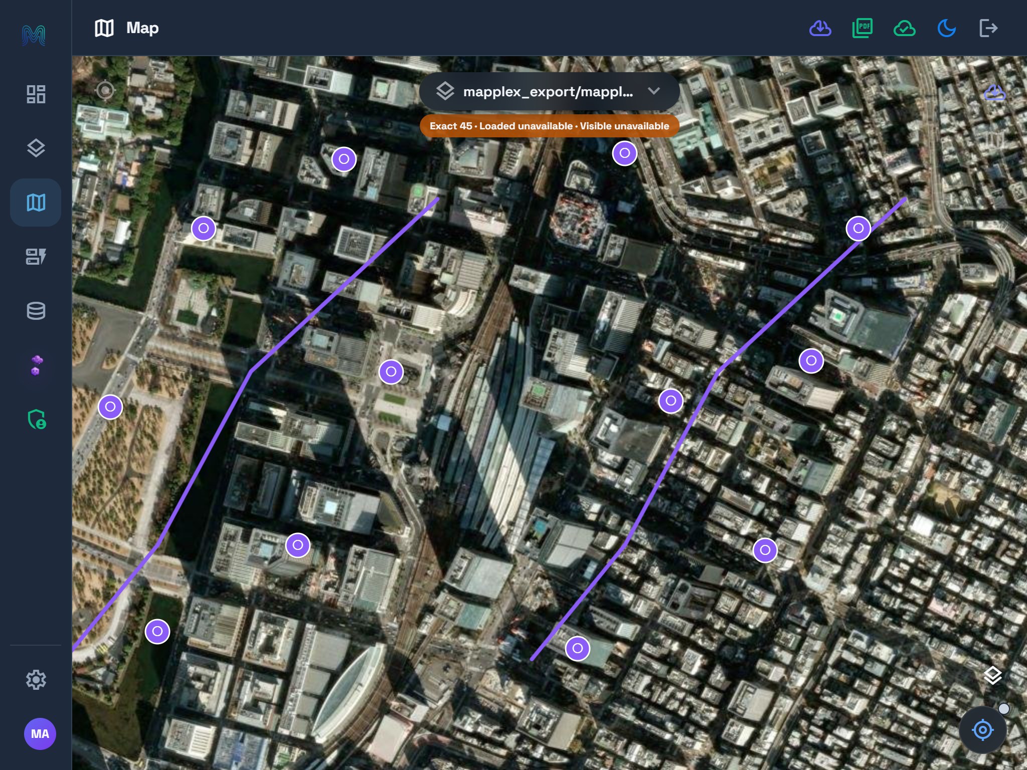
Choose Import Convertible CAD Entities (6). Wait for completion, then inspect the new layer in Data & Sync and on Map. The example creates MAPPLEX_EXPORT LineString Vector with six routes. Pan to Tokyo and compare the route placement with the source project.

The imported coordinates match the six source routes. Default import styling is used; the original GIS form and route attributes were not restored.

CAD Manager accepts DXF, not a DWG file renamed to DXF. Conversion supports common point, line and polygon-like entities, but it simplifies some CAD content: block inserts become insertion points, text becomes point attributes, and curves may be approximated. Inspect the imported result before relying on complex drawings. Source entity counts and resulting feature counts need not always be identical.

6. Export a shapefile package

Return to Global Field Operations. Open Data & Sync → SHP → Export SHP and select Entire Project in that manager. Choose Export as SHP.

A whole-project export is separated by geometry type inside the ZIP.

The ZIP contains 39 points, six lines and six polygons. Each group’s geometry and attribute record counts were checked.

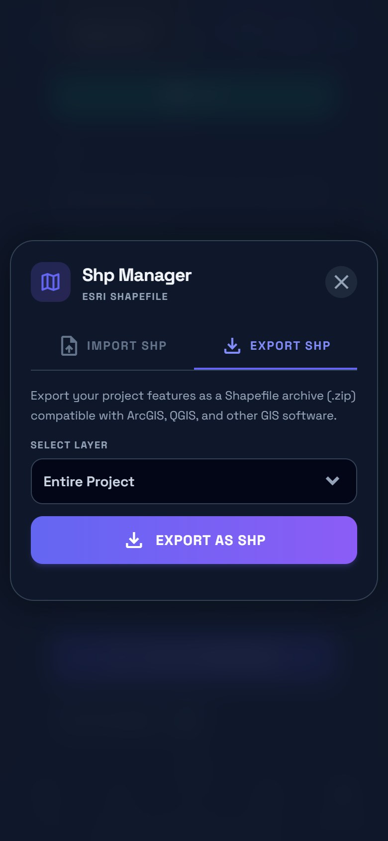
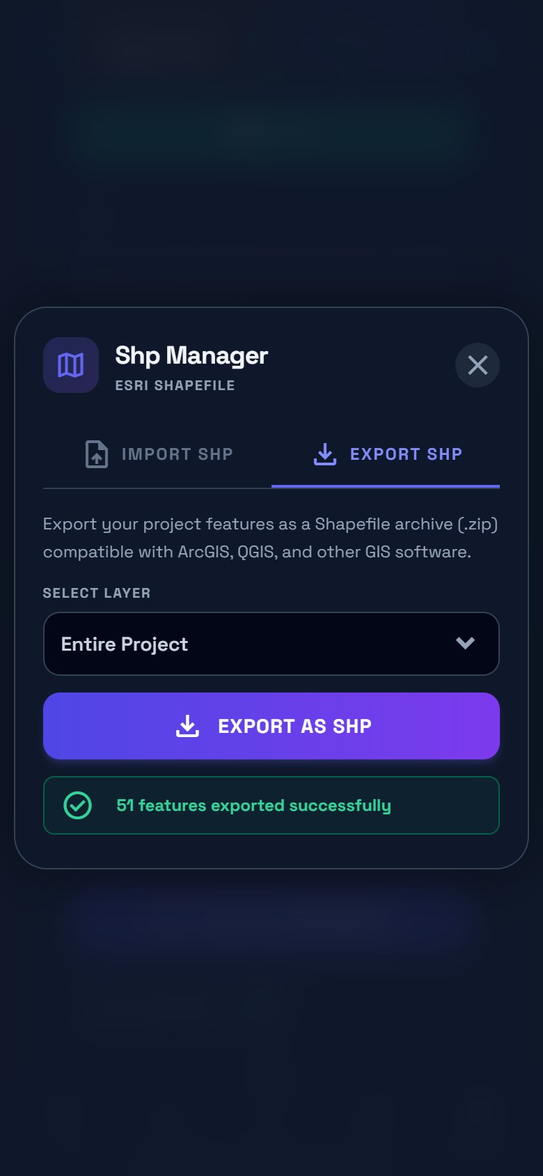
Keep the full ZIP. Each geometry group contains .shp geometry, .shx index, .dbf attributes, .prj coordinate-system information and .cpg text-encoding information. This exporter writes WGS84 coordinates and declares UTF-8.

The archive also includes mapplex-shapefile-schema.json, which records field-name and null-value mappings for Mapplex's ZIP import. DBF names are limited to ten characters: for example, Service zone becomes Service_zo. Other GIS software may show those shortened names rather than interpreting the Mapplex metadata.

SHP is a geometry-and-attributes exchange format, not a full restoration of forms, Lexicons, styling, relationships or attachments. If a field exceeds the supported DBF width or numeric precision, the exporter reports the problem; use GeoPackage or GeoJSON rather than assuming the value was preserved.

7. Preview and select the SHP data to import

Activate Global Exchange Lab again. Open Data & Sync → SHP → Import SHP and choose the ZIP. The preview lists the Points, Lines and Polygons datasets, their fields, feature counts and detected projection.

For this exercise, leave only the _points dataset checked: 39 features. The lab already has the six routes from DXF, so this selection adds the inspections without importing another route copy.

Only Points is checked, so the button shows **Import 39 Features (1 layer)**. Unchecked routes and polygons are excluded from this import.

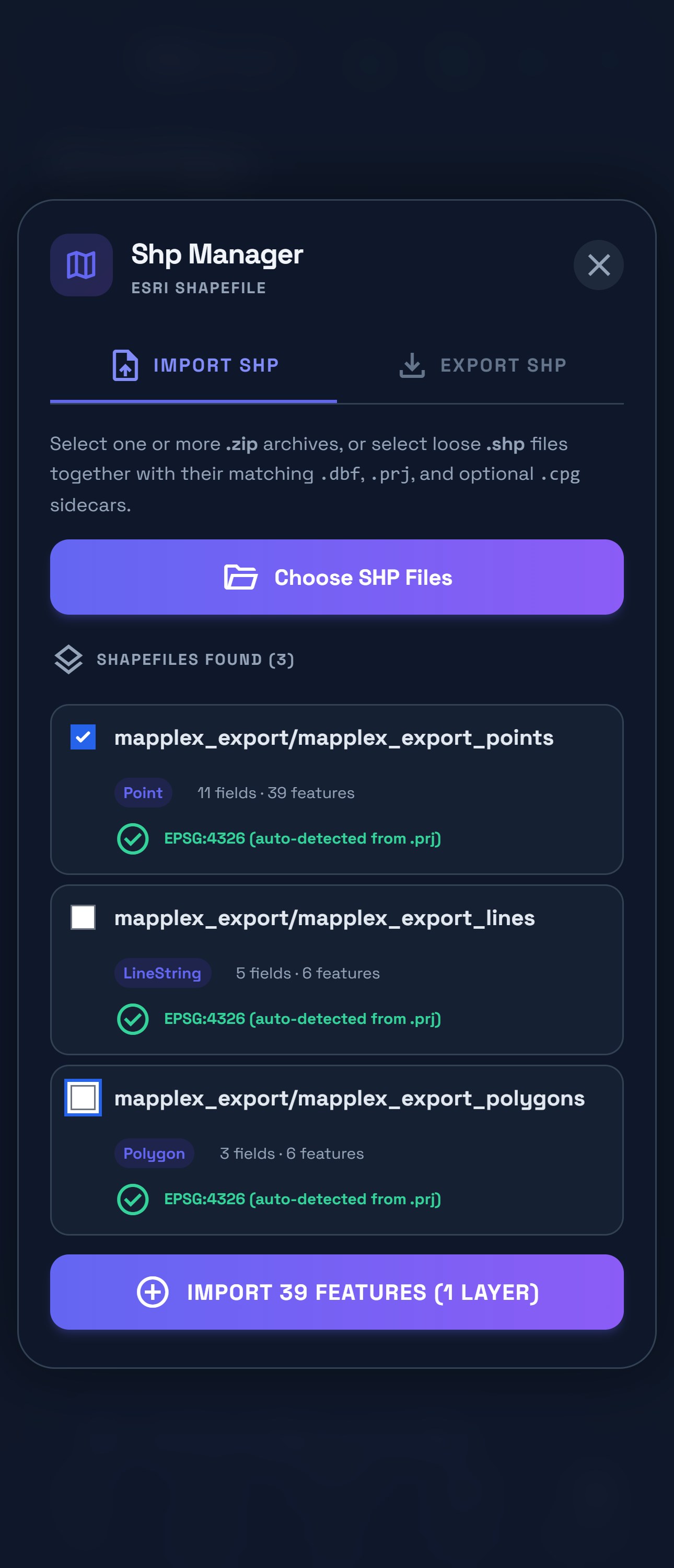
See the tablet mode view

All three datasets have EPSG:4326 detected from their .prj files. The preview was reopened for this image without importing a second copy.

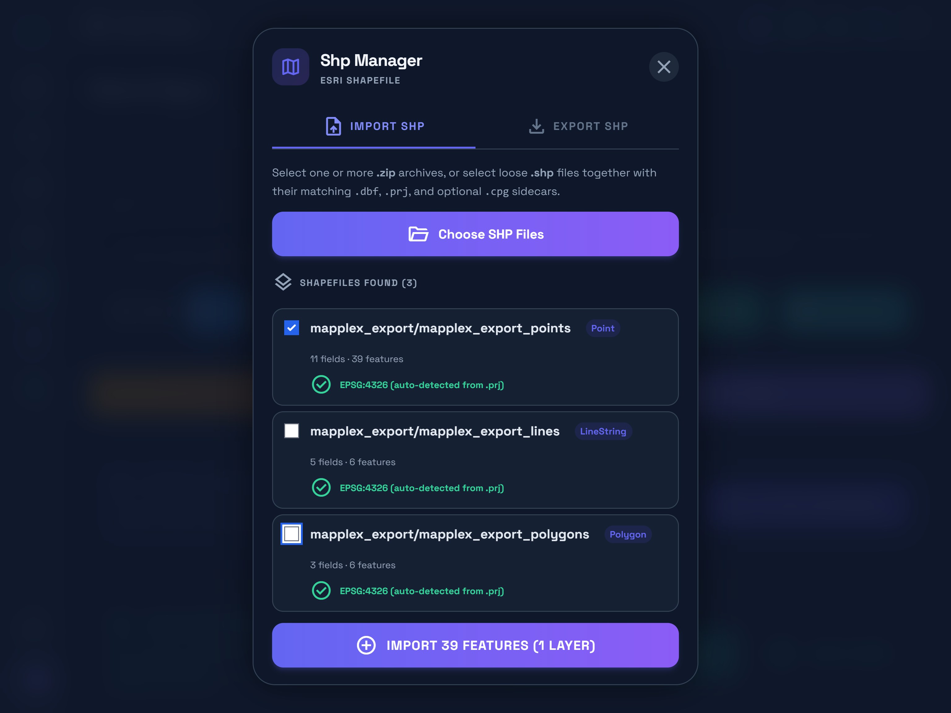
Check the selection, then verify the result

The import button updates to match the checked datasets. With only Points selected, expect 39 features (1 layer); with nothing selected, the button is disabled. The original exercise added 39 points, confirmed by reading the local records afterward. These refreshed previews were closed without importing another copy.

Choose the import button and wait for completion. When using loose files instead of a ZIP, select the .shp together with the matching .dbf (attributes), .shx (index) and .prj (coordinate system) files. Keep their base filenames aligned. If no usable .prj is available, establish the source CRS before using the manual CRS options; coordinates that merely look plausible are not sufficient.

8. Check the imported attributes and map

Expand the new points layer in Data & Sync and find LDN-013. Check Good, height 7.2, City london, Service zone London West, the note and inspection date. The import creates a form from the received fields; its internal field keys may differ from the source project's keys.

The original sample values survived this SHP export and import. The local lab contains 39 points plus six CAD routes: 45 features.

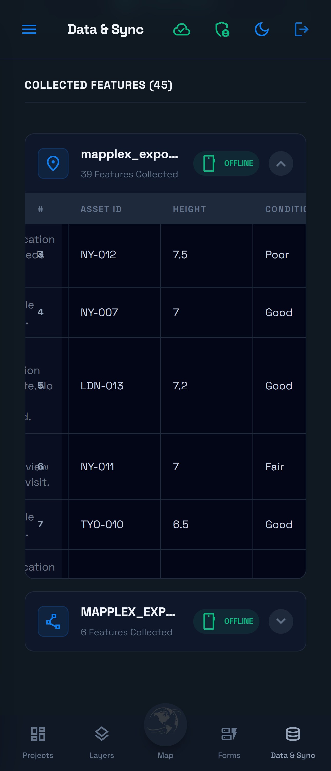
Open Map and review the imported layers around Tokyo, then New York and London. The geometry checks matched all six CAD routes and all 39 SHP points to their source coordinates within numerical rounding tolerance. Verify the intended field values and default styles before using a converted layer for new collection.

See the tablet mode view

The tablet view makes the imported point and route context visible together. Loaded or Visible unavailable remains a separate display diagnostic; the layer records were checked directly.

Download the Part 4 DXF and SHP practice files. The bundle includes the two app-generated exports, expected counts and validation notes. Extract the outer bundle, then select the DXF or inner shapefile ZIP in its manager.

These examples verify one standard capture and a focused exchange of sample geometry and attributes. They do not establish compatibility with every CAD drawing or external GIS application. See the format preservation reference for delivery requirements.

Before you continue

LDN-013 is saved through the standard form. Global Field Operations has 39 sites / 51 features. The separate Global Exchange Lab has 45 local copies: 39 SHP points and 6 CAD routes. Return to Projects and activate Global Field Operations before the optional AI exercises.

Previous: Part 3 · Review, sync and deliver · Learning path & counts · Optional: Geova AI review and questions